Understanding how database indexes work and how to use them efficiently !

Hello Readers,

Hope you are doing well! Today I m here with another interesting topic related to databases indexes. We all know like we use indexes to make our read operation faster but do we really take proper use and benefit of indexes?

We will check all the things in this blog. If you are new here and really wanna know about indexes and how it works internally you can check my previous blog.

We will be using PostgreSQL for all queries and demonstration parts.

So let's say we have a table named "test" with three attributes.

I have some random data in all three attributes lets check how much data is in our table

So we have around like 30K data. So just let's run our simple query to create an index on column (a) and on-column (b)as we know it will make our read operation faster.

Let's quickly verify our indexes if it has been created or not

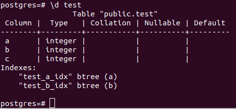
So yeah here we can see we have indexes that have been created properly. Let's run some SELECT queries and see how it behaves over indexes.

It's a simple query where we are trying to fetch column "c" data after applying conditions on column "a". We are using explain analyze syntax here its simply executes the query and tells us the cost of the query.

Let's understand what it's telling us we will start from innermost then move to outermost. Let's break it down into two parts one part for the index data structure and one part for the actual table.

Index operations

• Index Cond: (a = 70): - This is basically the where condition we have specified in our query so while scanning via index data structure it's taking the help our where condition

• (cost=0.00..4.30 rows=2 width=0):- The first value of the cost variable i.e.; 0.00 is telling us how much time(milliseconds) it takes to fetch the first page from the HDD. (If you want to know how databases store their data you can visit my previous blog.) and a second value of the cost variable i.e.; 4.30(milliseconds) tells us how much time it takes to fetch the last page from HDD. The rows variable tells us how many rows it fetched from the index data structure.

• (actual time=0.027..0.027 rows=2 loops=1):- Now after this the actual time variable telling us how much actual time it takes to perform this scanning on the index data structure. The rows variable tells us how many rows or memory blocks is fetched from the index data structure. The loops variable tells us how many loops it has been used to find the value 70 i.e.; our where condition.

• Bitmap Index Scan on test_a_idx:- This tells us that the query planner decided to use bitmap index scan on the index data structure name as test_a_idx. (The index we created on column a).

• Heap Blocks: exact=2:- This describes exactly two blocks that are mapped and fetched from the heap table.

• Recheck Cond: (a=70):- This describes that after fetching the actual data from the heap table we again recheck the condition.

• Bitmap Heap Scan on the test (cost=4.31..11.83 rows=2 width=4):- The first value of the cost variable i.e.; 4.31 is telling us how much time(milliseconds) it takes to fetch the first page from the HDD after performing all the internal operations and mapping. The second value of the cost variable i.e.; 11.83(milliseconds) tells us how much time it takes to fetch the last page from HDD. The variable rows=2 tells us how many rows or memory blocks we actually fetched after performing operations. The width tells the actual size of the returned data as we are returning the "c" column and its data type is an integer so the returned value here will be 4.

Here's the question that arises in the above operation why it is using bitmap and what is a bitmap?

Let see what is bitmap! As we know PostgreSQL uses a secondary index for storing all the rows. Secondary index means it only stores the reference of the value in index data structure but the actual value gets stored in a heap table. We will not deep dive into this blog but if you want to know about this let me know in the comments section. :-). Let me present you with a sample image hope this helps.

In the above figure, you can see the actual value got clustered index but its reference got stored in the secondary index.

The bitmap index scan from the index data structure to get the reference of the records once it finds the reference it then it maps to the heap table to get the actual value. that's why there is a map word in its name.

So we have seen above how indexing is working. Now execute one more condition over-indexed columns with AND condition.

In the above condition, we can see it's still using bitmap index but if you see there are some extra gibberish coming up. Let's see the extra ones only the previous ones we have already covered.

• Bitmap Index Scan on test_a_idx:- This tells us that the query planner decided to use bitmap index scan on the index data structure name as test_a_idx.

• Bitmap Index Scan on test_b_idx:- This tells us that the query planner decided to use bitmap index scan on the index data structure name as test_b_idx.

• If you see here in order to perform fast fetching the PostgreSQL parallelly running two index operations on column a and column b

• And after both parallel operations is completed there result set gets combined to BitmapAnd

It is interesting to see how smart our query planner is! He knows when to do a parallel processes and when to do the sequential process. Meanwhile, query planner is like. :-)

Okay, jokes aside let's perform some more operations and see how indexes gonna work!

let's run the above query with the OR condition.

In this again there is the same operation as the above only thing that is changed is the number of rows that are going to return. As we are using OR condition so it's gonna return more rows.

Let's create a composite index and check how the index gonna work. So we just gonna write our beautiful index on the table test along with columns "a" and "b".

create index on test(a,b);

Let's run the same previous simple select query.

if you see here its perform the same operation as the previous one. Let's run the same query but on column "b" and see how it behaves.

Well well, why it is using sequential scan(Line by line scan not using the help of index) when I have already created an index on both columns "a" and as well as "b"?

yes my friend this is how the composite index works. Whenever you create a composite index it's always gonna use the left written column name when you write any condition with a single column. Suppose we do vice versa and write a statement

create index on test(b,a)

Then in this case the column "a" will start using sequential scan and column "b" will start using the index scan when you write any condition with a single column.

hmm, So now the question comes what benefit we will get with this composite index scan?

Let's run the query the same query with AND condition.

It's the same query as above but with index scan and we can see here a lot of gibberish has been gone and the query planner is only using index scan. there is no BitMap mapping no combining of two parallel queries just sweet and simple index scan. And if you see the execution time and compare the result. (Let me know in the comment section if you wanna know about different types of scan in databases :-) )

• With single index on both column(a,b) with same condition 0.118ms

• With composite index on both column(a,b) with same condition 0.044ms

Yes, my friend, this is the benefit we get by using a composite index. :-)

Let's use the OR query for the same and see the performance.

OMG! it using sequential scan and if you see the execution time its 15.892ms

Let's move on from the meme part. Now the question comes how we can optimize it in case we have created a compound index. What we can do is we can again create a single index on a single column "b".

Let's create the same on column "b" and again re-run the same OR query and see the performance.

Voila! Now our column "b" also started using the indexing mechanism and time is also get reduced. But if you see the cost here is, on two attributes you have created two different types of indexes i.e.; composite index on column (a,b) and then after again single index on column b. This will create an overhead of rearranging the index's position and it will consume more space.

The main motive to write this blog is just to tell you that if you are going to use indexes always think about your use case and then choose the best fit index creation technique.

So yeah that's all in this blog just a little bit of introduction and working on indexes. Please do read and share your feedback!

Keep Reading! Keep learning!